Extracted images: Stormwater Management Quantity and Quality Standards and Computations

Printed revision: July 2023.

Back to source | Original PDF | Image metadata

Original Mistral crops are preserved byte for byte. A crop can be a figure, table, equation, or other visual; no visual content is inferred as a numerical rule. Record and table associations use the same PDF page unless a direct image placeholder is identified. Nearby OCR excerpts are context, not verified captions.

PDF page 1, image 1

Mistral ID: img-0.jpeg. Extraction bundle(s): 2023_BMP_5_SWM_Standards_and_Computations. Original page | Image file

Surrounding OCR excerpt:

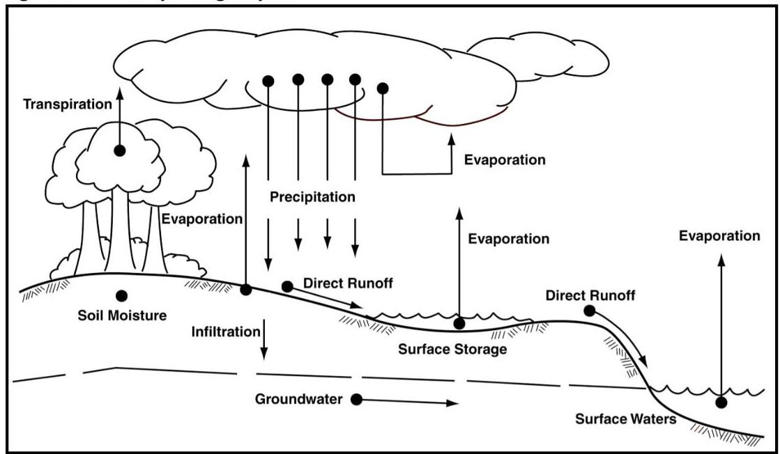
recipitates as rainfall can wind up, or at least spend time, on ground or plant surfaces, in the atmosphere, within the various soil layers or in waterways and water bodies.

Figure 5-1: The Hydrologic Cycle
[OCR image]
Source: Fundamentals of Urban Runoff Management.

The physical processes that convert rainfall to runoff are both complex and highly variable. As such, these processes cannot be replicated mathematically with exact certainty. However, by making simplifying

PDF page 4, image 1

Mistral ID: img-1.jpeg. Extraction bundle(s): 2023_BMP_5_SWM_Standards_and_Computations. Original page | Image file

Surrounding OCR excerpt:

s for the same storm events.

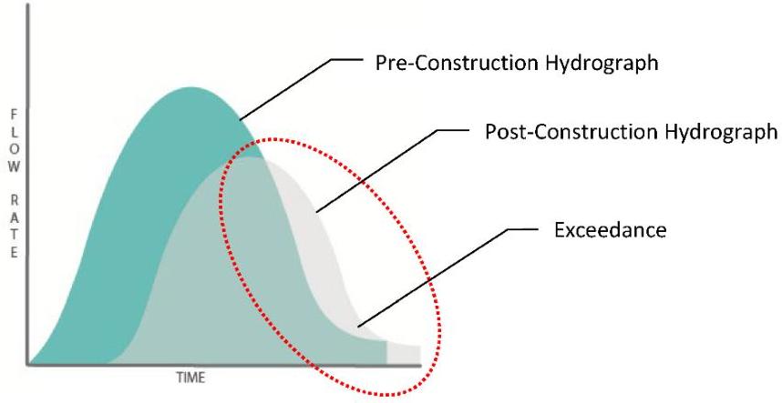
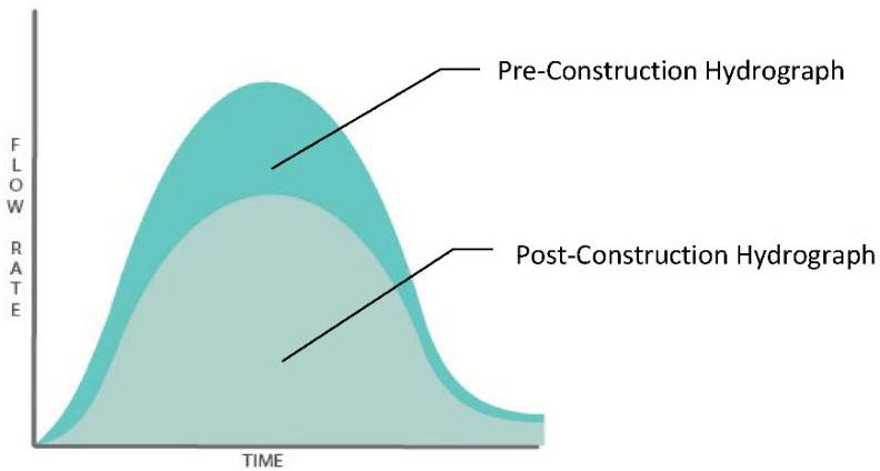
Below is Figure 5-2, which is an illustration demonstrating noncompliance with the requirement under N.J.A.C. 7:8-5.6(b)1, followed by Figure 5-3 which demonstrates compliance:

[OCR image]
Figure 5-2: Post-Construction Hydrograph Exceeds the Pre-construction Hydrograph

In the preceding graphic, the peak of the post-construction hydrograph, shown in grey, is lower than the peak of the pre-construction hydrograph, shown in teal, and some points of the post-construction hydrograph lie outside the pre-construction hydrograph, shown within the dashed

PDF page 5, image 1

Mistral ID: img-2.jpeg. Extraction bundle(s): 2023_BMP_5_SWM_Standards_and_Computations. Original page | Image file

Surrounding OCR excerpt:

oval area; therefore, the post-construction hydrograph does not meet the requirements set forth at N.J.A.C. 7:8-5.6(b)1.

[OCR image]
Figure 5-3: Post-Construction Hydrograph does not Exceed the Pre-construction Hydrograph at any Point

In Figure 5-3, the post-construction hydrograph meets the aforementioned requirement since every point of the post-construction hydrograph is under the pre-construction hydrograph.

It is important to note that the area under the hydrograph represents the volume of the stormwater runoff. In order to co

PDF page 12, image 1

Mistral ID: img-3.jpeg. Extraction bundle(s): 2023_BMP_5_SWM_Standards_and_Computations. Original page | Image file

Surrounding OCR excerpt:

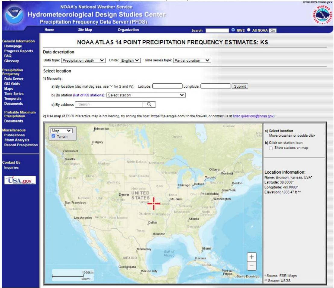
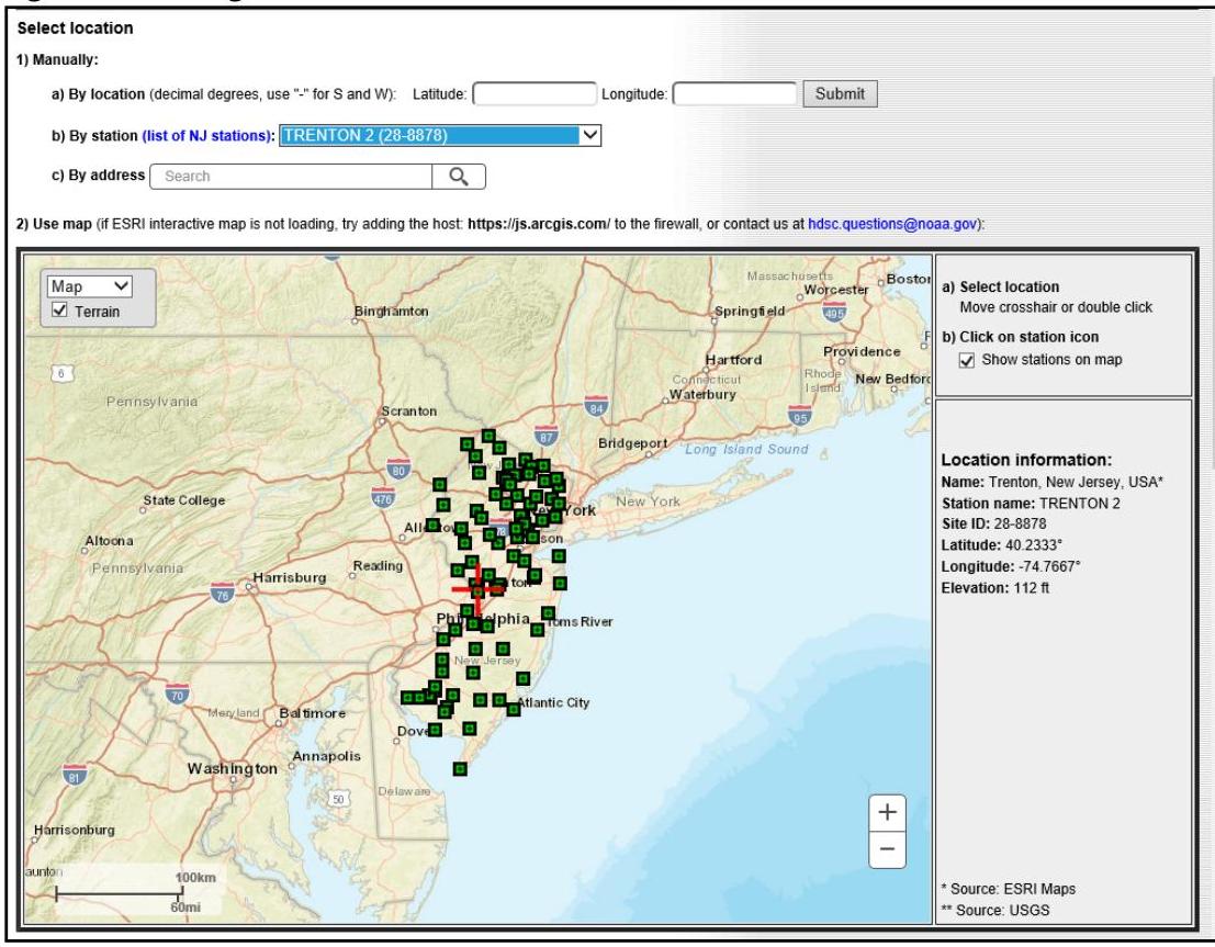
Step 1: Under the Select location option, depicted in Figure 5-4 below, manually enter the location using one of the options offered on the screen or use the map to locate the site, making sure to zoom in.

[OCR image]
Figure 5-4: NOAA's NWS Precipitation Frequency Data Server Website

PDF page 13, image 1

Mistral ID: img-4.jpeg. Extraction bundle(s): 2023_BMP_5_SWM_Standards_and_Computations. Original page | Image file

Tables on the same PDF page: Table 3

Surrounding OCR excerpt:

ype: Precipitation depth | Units: English | Time series type: Partial duration  |

To illustrate this process, Trenton Station 2 was selected from the dropdown menu under 1.b), as shown in Figure 5-6 below:

[OCR image]
Figure 5-6: Using Manual Location Selection on the NOAA NWS PFDS Website

Step 3: Scroll down the page to the Point Precipitation Frequency (PF) Estimates section. Left click on the PF tabular option, if it does not appear on top of the other tabs, which will be shaded in dark blue, as shown in Figure 5-7.

PDF page 14, image 1

Mistral ID: img-5.jpeg. Extraction bundle(s): 2023_BMP_5_SWM_Standards_and_Computations. Original page | Image file

Surrounding OCR excerpt:

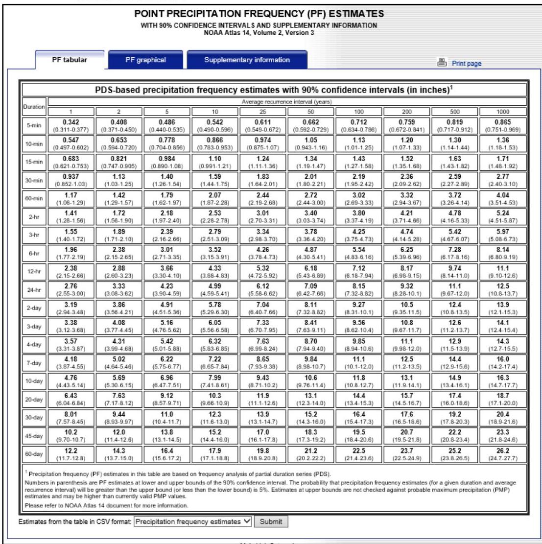
Figure 5-7: Point Precipitation Frequency (PF) Estimates – Tabular Option for Trenton Station 2

[OCR image]

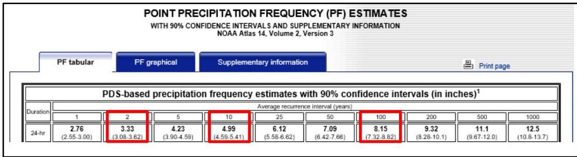
The data needed is found in the row labeled "24-hr." The values in the columns labeled "2," "10" and "100" correspond to the rainfall depths generated by the 2-, 10- and 100-year design storms, respectively, for this weather station location, as outlined in red in Figure 5-8 below.

Figure 5-8: Locating the 2-, 10- and 100- year Design Storm Rainfall Data for Trenton Station 2

![img-6.jpeg](img-6.jpeg

PDF page 14, image 2

Mistral ID: img-6.jpeg. Extraction bundle(s): 2023_BMP_5_SWM_Standards_and_Computations. Original page | Image file

Surrounding OCR excerpt:

-year design storms, respectively, for this weather station location, as outlined in red in Figure 5-8 below.

Figure 5-8: Locating the 2-, 10- and 100- year Design Storm Rainfall Data for Trenton Station 2

[OCR image]

PDF page 20, image 1

Mistral ID: img-7.jpeg. Extraction bundle(s): 2023_BMP_5_SWM_Standards_and_Computations. Original page | Image file

Surrounding OCR excerpt:

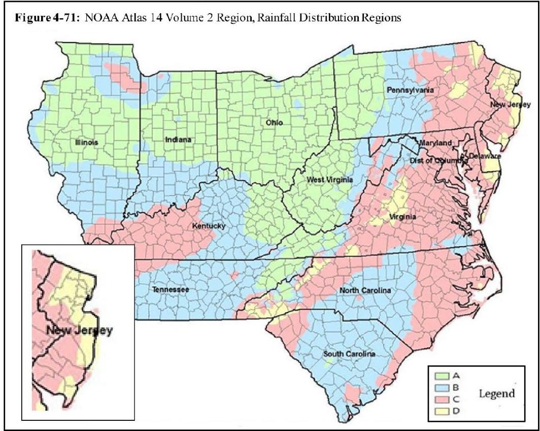
as shown in Figure 5-9. This figure is a reprint of Figure 4-71 in Chapter 4 of the NEH and is found online at the link below:

https://directives.sc.egov.usda.gov/OpenNonWebContent.aspx?content=43924.wba.

[OCR image]
Figure 5-9: NJ Locations of Regions C and D

The updated extents of Regions C and D shown in Figure 5-9, and either shaded in orange or yellow, indicate that both Rainfall Distribution Regions C and D may not follow the county boundaries as stated in the NEW JERSEY BULLETIN NO. NJ210-12-1. If a project is near a rainfall distribution region boundary, it might be difficult to identify the respective rain

PDF page 21, image 1

Mistral ID: img-8.jpeg. Extraction bundle(s): 2023_BMP_5_SWM_Standards_and_Computations. Original page | Image file

Surrounding OCR excerpt:

vel of stormwater pollution control.

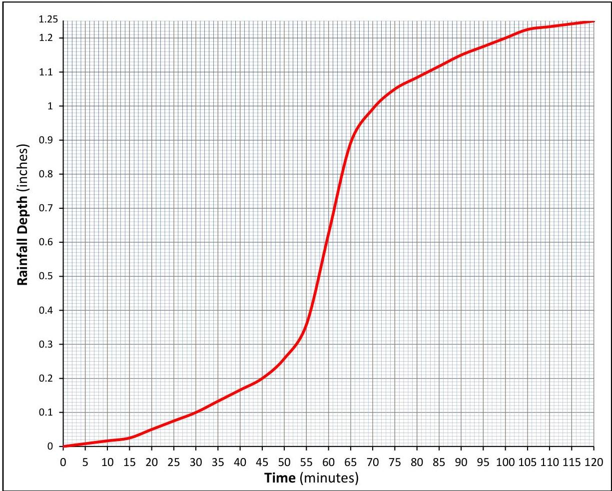
The accumulative distribution curve for rainfall depth, shown in Figure 5-10, is a graphical representation of 1.25 inches of rainfall falling in the 2-hour NJDEP WQDS.

[OCR image]
Figure 5-10: Stormwater Runoff Water Quality Design Storm Rainfall Cumulative Distribution Curve

An Excel file providing the rainfall distribution and rainfall intensity of the WQDS, in 1 minute intervals, is also available on the Department's website, under the heading for Chapter 5, via the following link:

https://www.njstormwater.org/bmp_manual2.htm

PDF page 23, image 1

Mistral ID: img-9.jpeg. Extraction bundle(s): 2023_BMP_5_SWM_Standards_and_Computations. Original page | Image file

Surrounding OCR excerpt:

[OCR image]
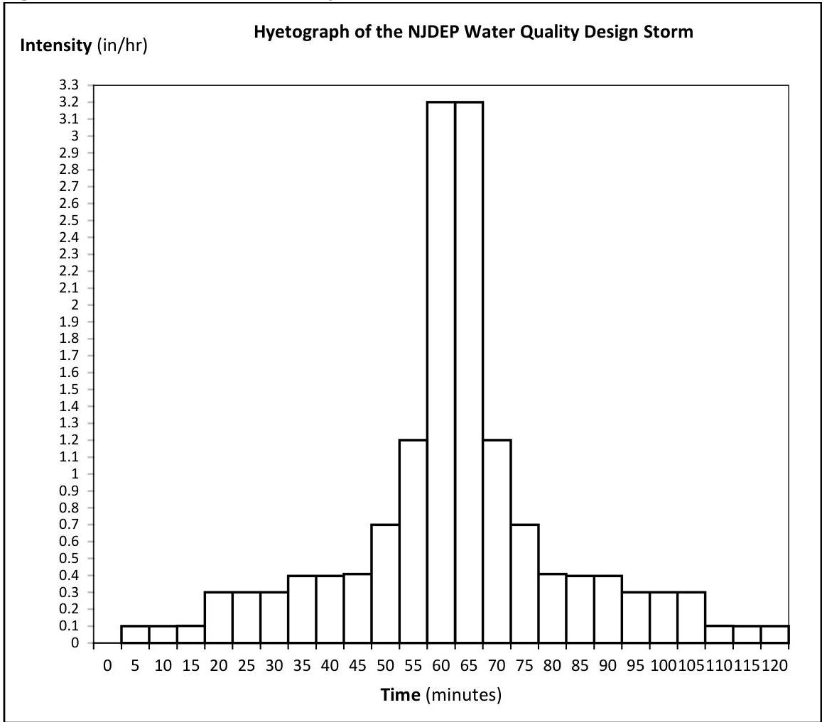
Figure 5-11 depicts the intensity of the rainfall distribution derived from Table 5-2.
Figure 5-11: WQDS Rainfall Intensity Distribution

8. The time of travel and the time of concentration: One of the methods identified in the NRCS methodology for calculating time of concentration  $(T_{c})$  is the velocity method, which assumes the time of concentration is "the sum of travel times for segments along

PDF page 26, image 1

Mistral ID: img-10.jpeg. Extraction bundle(s): 2023_BMP_5_SWM_Standards_and_Computations. Original page | Image file

Surrounding OCR excerpt:

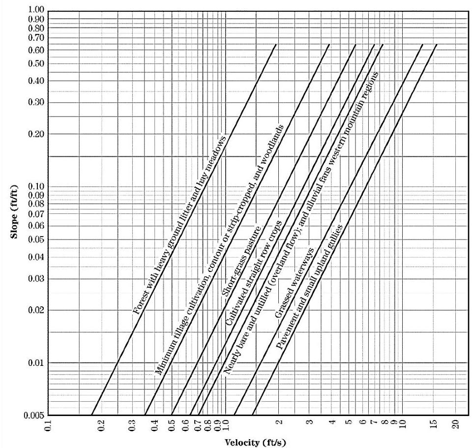
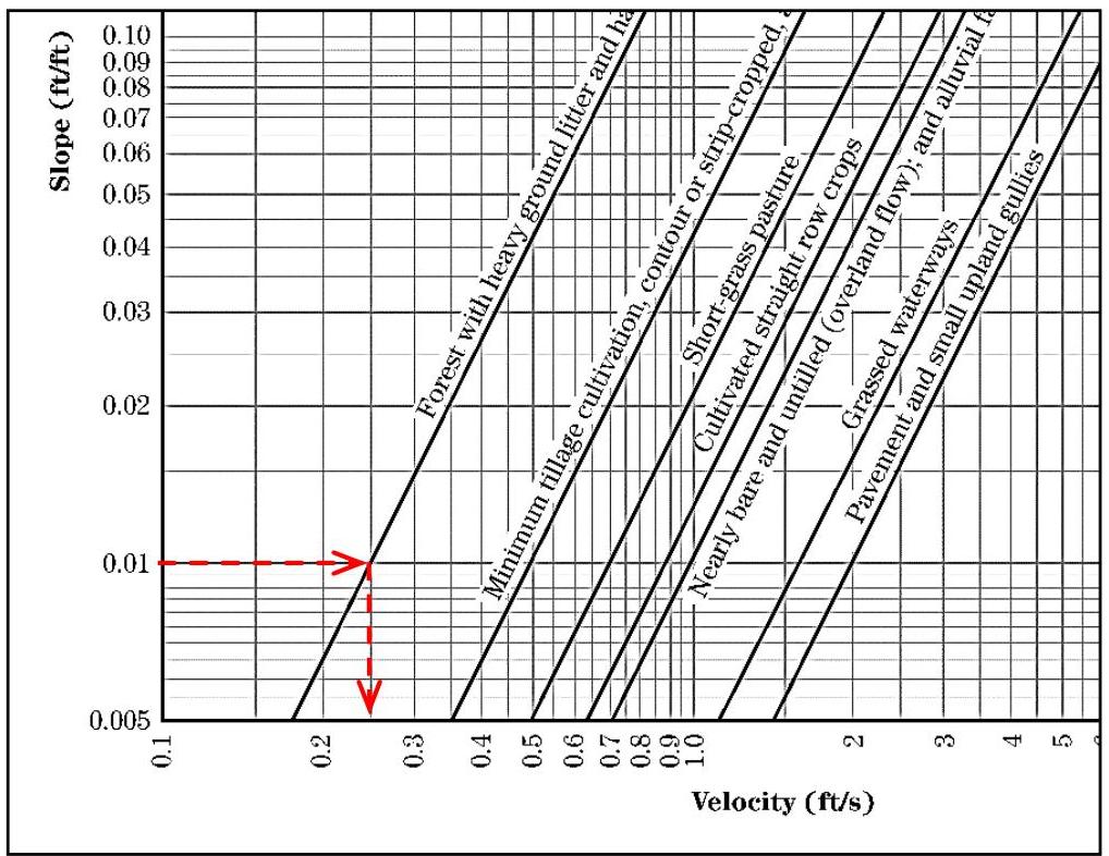
Figure 5-13: Velocity Versus Slope for Shallow Concentrated Flow From NEH, Part 630, Chapter 15
[OCR image]
Figure 15-4 Velocity versus slope for shallow concentrated flow

For this type of flow, the average velocity of the flow in the segment must be derived from Figure 15-4 in NEH and then input into Equation 15-1 to calculate the travel time:

$$
T _ {t} = \frac {\text {Shallow Concentrated Flow Length}}{V \times 3600}
$$

where  $T_{t}$  is the travel time (hr) and  $V$  is the average flow velocity (ft/

PDF page 28, image 1

Mistral ID: img-11.jpeg. Extraction bundle(s): 2023_BMP_5_SWM_Standards_and_Computations. Original page | Image file

Surrounding OCR excerpt:

[OCR image]
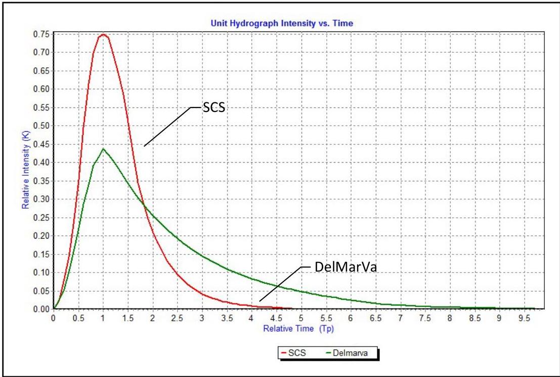
Figure 5-14: NRCS Standard DUH (484 DUH) versus the DelMarVa DUH

The DelMarVa DUH must be used in calculating pre-construction peak flowrates for the 2-, 10- and 100-year storms in the Coastal Plain Region of New Jersey, unless the design engineer proves, to the satisfaction of the review engineer, that the conditions for applicability are not present anywhere in the watershed. The physiographic provi

PDF page 29, image 1

Mistral ID: img-12.jpeg. Extraction bundle(s): 2023_BMP_5_SWM_Standards_and_Computations. Original page | Image file

Surrounding OCR excerpt:

[OCR image]
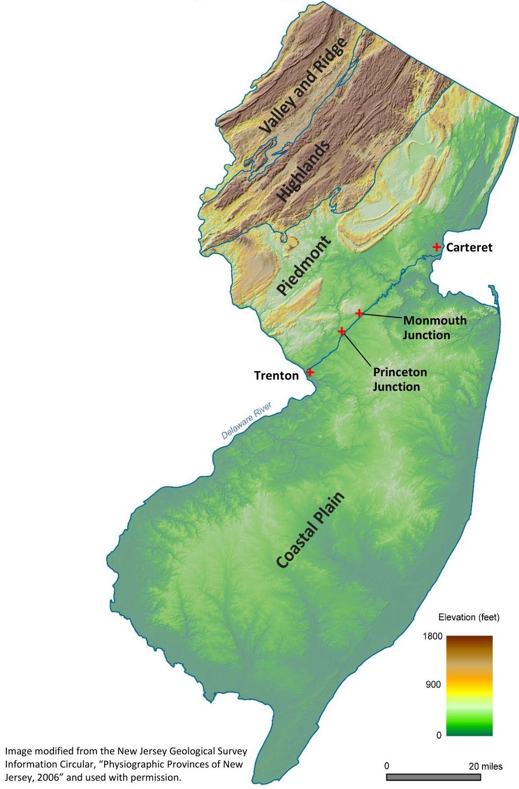
Figure 5-15: Physiographic Provinces of NJ

PDF page 30, image 1

Mistral ID: img-13.jpeg. Extraction bundle(s): 2023_BMP_5_SWM_Standards_and_Computations. Original page | Image file

Surrounding OCR excerpt:

ge system, water bodies and riparian zones or wetlands.
b. Runoff is shallow concentrated flow that runs over a pervious area and then into the drainage system, water bodies and riparian zones or wetlands.

[OCR image]
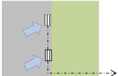
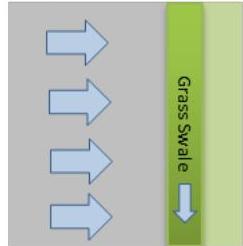
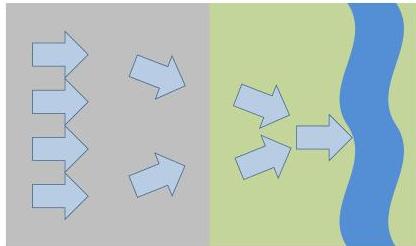
Figure 5-16: Directly Connected Impervious Surfaces
Connected to Stormwater
Collection System

[OCR image]
Connected to
Down-gradient BMP

[OCR image]
Concentrated Flow Directed to
Down-gradient Stream

Shown above are examples of directly connected impervious surfaces, which include, but are not limited to, runoff from an impervious surface

- collected by a storm drain

PDF page 30, image 2

Mistral ID: img-14.jpeg. Extraction bundle(s): 2023_BMP_5_SWM_Standards_and_Computations. Original page | Image file

Surrounding OCR excerpt:

ea and then into the drainage system, water bodies and riparian zones or wetlands.

[OCR image]
Figure 5-16: Directly Connected Impervious Surfaces
Connected to Stormwater
Collection System

[OCR image]
Connected to
Down-gradient BMP

[OCR image]
Concentrated Flow Directed to
Down-gradient Stream

Shown above are examples of directly connected impervious surfaces, which include, but are not limited to, runoff from an impervious surface

- collected by a storm drain, which then connects to a conduit or channel to a downstream BMP, stormwater collection system or stream or
- flowing over

PDF page 30, image 3

Mistral ID: img-15.jpeg. Extraction bundle(s): 2023_BMP_5_SWM_Standards_and_Computations. Original page | Image file

Surrounding OCR excerpt:

ian zones or wetlands.

[OCR image]
Figure 5-16: Directly Connected Impervious Surfaces
Connected to Stormwater
Collection System

[OCR image]
Connected to
Down-gradient BMP

[OCR image]
Concentrated Flow Directed to
Down-gradient Stream

Shown above are examples of directly connected impervious surfaces, which include, but are not limited to, runoff from an impervious surface

- collected by a storm drain, which then connects to a conduit or channel to a downstream BMP, stormwater collection system or stream or
- flowing over a pervious surface by shallow concentrated flow or channeli

PDF page 31, image 1

Mistral ID: img-16.jpeg. Extraction bundle(s): 2023_BMP_5_SWM_Standards_and_Computations. Original page | Image file

Surrounding OCR excerpt:

help provide both groundwater recharge and stormwater quality treatment for small rainfall events as well as reduce the overall runoff volume that must be treated and/or controlled in a down-gradient BMP.

[OCR image]
Figure 5-17: Unconnected Impervious Surfaces

[OCR image]

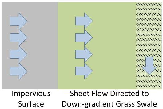
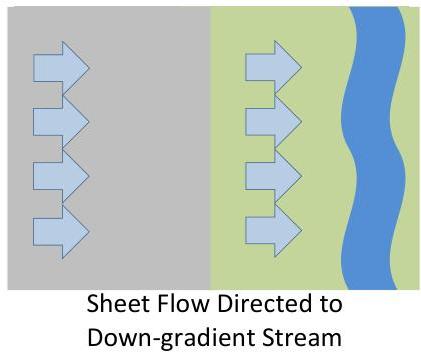
An impervious area can be considered to be an unconnected impervious surface only when meeting all of the following conditions:

a. Upon entering the down-gradient pervious area, all runoff must remain as sheet flow.
b. Flow from the impervious surface must enter the down-gradient pervious area as sheet flow or, in the case of r

PDF page 31, image 2

Mistral ID: img-17.jpeg. Extraction bundle(s): 2023_BMP_5_SWM_Standards_and_Computations. Original page | Image file

Surrounding OCR excerpt:

or small rainfall events as well as reduce the overall runoff volume that must be treated and/or controlled in a down-gradient BMP.

[OCR image]
Figure 5-17: Unconnected Impervious Surfaces

[OCR image]

An impervious area can be considered to be an unconnected impervious surface only when meeting all of the following conditions:

a. Upon entering the down-gradient pervious area, all runoff must remain as sheet flow.
b. Flow from the impervious surface must enter the down-gradient pervious area as sheet flow or, in the case of roofs, from one or more downspouts, each equipped with a splash pad, level

PDF page 35, image 1

Mistral ID: img-18.jpeg. Extraction bundle(s): 2023_BMP_5_SWM_Standards_and_Computations. Original page | Image file

Surrounding OCR excerpt:

[OCR image]

The corresponding velocity is 0.25 ft/s. This value is then entered into the equation for the travel time, as follows:

$$
T _ {t} = \frac {9 8 5 . 0 0}{0 . 2 5 \times 3 6 0 0} = 1. 0 9 \mathrm {h r} = 6 5. 5 \mathrm {m i n}
$$

Step 3: Since no channel flow is specified in the example, the time of concentration for the post-construction condition is the sum of the travel times under sheet flow and sh

PDF page 36, image 1

Mistral ID: img-19.jpeg. Extraction bundle(s): 2023_BMP_5_SWM_Standards_and_Computations. Original page | Image file

Surrounding OCR excerpt:

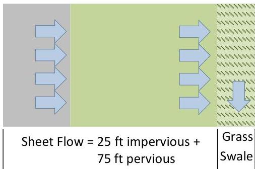
24 hours. The slope of the impervious surface and the grass lawn area are each at 1%. From Table 9-5, in NEH Part 630, Chapter 9, a lawn area in HSG 'A' soil has a Curve Number of 39, under good condition.

[OCR image]

## Step 1: Calculate the Percentage of Total Impervious Surface

To use the NRCS composite CN with unconnected impervious area method, one must first calculate the percentage of the total impervious area to the total area. The percentage of the total impervious surface to the total area is

$$
= (200 \text{ ft} \times 25 \text{ ft}) / [(200 \text{ ft} \times 25 \text{ ft}) + (200 \text{ ft} \times 75

PDF page 37, image 1

Mistral ID: img-20.jpeg. Extraction bundle(s): 2023_BMP_5_SWM_Standards_and_Computations. Original page | Image file

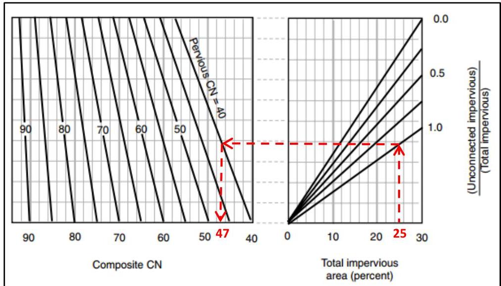
Surrounding OCR excerpt:

h is approximately 47. Take care reading the x-axis as the values increase from right to left. Therefore, a Curve Number = 47 can be used to represent the entire area measuring 200 ft wide and 100 ft long.

[OCR image]
Source: Figure 9-4, NEH, Part 630, Chapter 9

# Step 4: Use the Composite CN from Step 3 in the Runoff Depth Calculation

The depth of runoff will be calculated by Equation 10-11 in Chapter 10 of NEH, Part 630, as follows,

$$
Q = \frac {(P - 0 . 2 S) ^ {2}}{(P + 0 . 8 S)}
$$

where:

$Q =$  runoff, in

$P =$  rainfall, in  $= 3.5$  in

$S = \frac{1000}{CN} - 10 = \frac{1000}{47} - 10 = 11.3$ , using t

PDF page 38, image 1

Mistral ID: img-21.jpeg. Extraction bundle(s): 2023_BMP_5_SWM_Standards_and_Computations. Original page | Image file

Surrounding OCR excerpt:

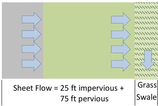
# Example 5-3: Use the NJDEP Two-Step Method for an Unconnected Impervious Surface to calculate the runoff volume for a site

[OCR image]

As can be surmised from the name, this method requires a two-step technique using the initial abstraction provided by NRCS runoff equation. First the volume of runoff generated by just the impervious area is calculated and then this volume is considered as if it were additional rain falling on the pervious area. The design storm event illustrated is the current 2-year storm, in which the current rainf

PDF page 39, image 1

Mistral ID: img-22.jpeg. Extraction bundle(s): 2023_BMP_5_SWM_Standards_and_Computations. Original page | Image file

Surrounding OCR excerpt:

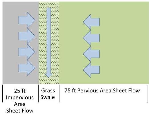
s belonging to HSG 'A.' The storm event of concern is the 2-year storm, in which 3.5 in of rain falls over a period of 24 hours. The slopes of the impervious surface and the grass lawn are each $1\%$. From

[OCR image]

Table 9-5 in Chapter 9 of NEH, Part 630, the grass lawn area specified has a Curve Number of 39.

A value of 98 is used as the CN value for impervious surfaces. If a weighted composite CN were applied in this situation, the weighted composite CN would be calculated as follows:

$$
CN = \frac{98 \times (200 \text{ ft} \times 25 \text{ ft}) + 39 \times (200 \text{ ft} \times 75 \text{ ft})}{(200 \text{

PDF page 41, image 1

Mistral ID: img-23.jpeg. Extraction bundle(s): 2023_BMP_5_SWM_Standards_and_Computations. Original page | Image file

Surrounding OCR excerpt:

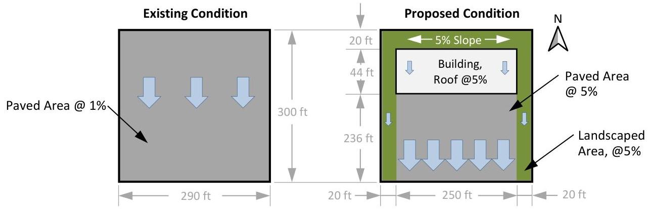
east and west sides of the proposed development, and each area also slopes from north down to the south. The landscaped area will not receive runoff from the impervious surfaces. HSG 'C' soils are present.

[OCR image]
Step 1: Calculate the current rainfall depths and the projected rainfall depths for the 2-, 10- and 100-year storms for the site.

The NOAA rainfall data was obtained in Example A-1. In the following table, the respective current precipitation adjustment factors and future precipitation change factors for Mercer County are applied as required to obtain the precipitation depths for current and projected

PDF page 43, image 1

Mistral ID: img-24.jpeg. Extraction bundle(s): 2023_BMP_5_SWM_Standards_and_Computations. Original page | Image file

Tables on the same PDF page: Table 15

Surrounding OCR excerpt:

nge factor to the NOAA NWS PFDS rainfall data, are depicted below. The hydrographs were created by exporting the hydrograph tables as CSV data and then using a spreadsheet program to graph the information.

[OCR image]

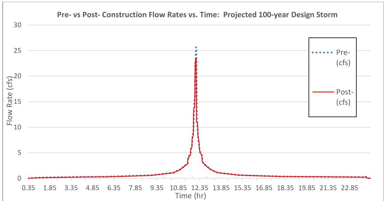
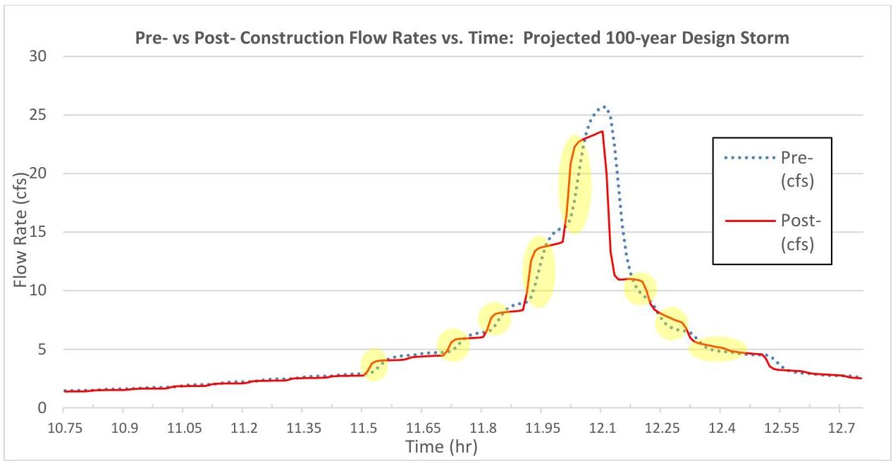
At first glance, one might assume the difference is negligible. However, the Rules do not permit any exceedance. If one were to zoom in on the previous hydrograph, e.g., starting at 11.92 hours, one would see the post-construction hydrograph has a higher flow rate than the pre-construction hydrograph in certain time periods. Some of these exceedances are highlighted in yellow in the following graphic.

PDF page 44, image 1

Mistral ID: img-25.jpeg. Extraction bundle(s): 2023_BMP_5_SWM_Standards_and_Computations. Original page | Image file

Tables on the same PDF page: Table 16

Surrounding OCR excerpt:

[OCR image]

A portion of the hydrograph data is also listed in the table below, for which the exceedances are highlighted in yellow. Take note this is just one example of two clusters of exceedances for this storm.

|  Time (hr) | Pre-construction (cfs) | Post-construction (cfs) | Difference in Flow Rate, Post - Pre, (cfs)  |
| --- | --- | --- | --- |
|  11.91 | 9.04 | 9.86 | 0.82  |
|  11.92 | 9.44 | 12.52 | 3.0

PDF page 46, image 1

Mistral ID: img-26.jpeg. Extraction bundle(s): 2023_BMP_5_SWM_Standards_and_Computations. Original page | Image file

Surrounding OCR excerpt:

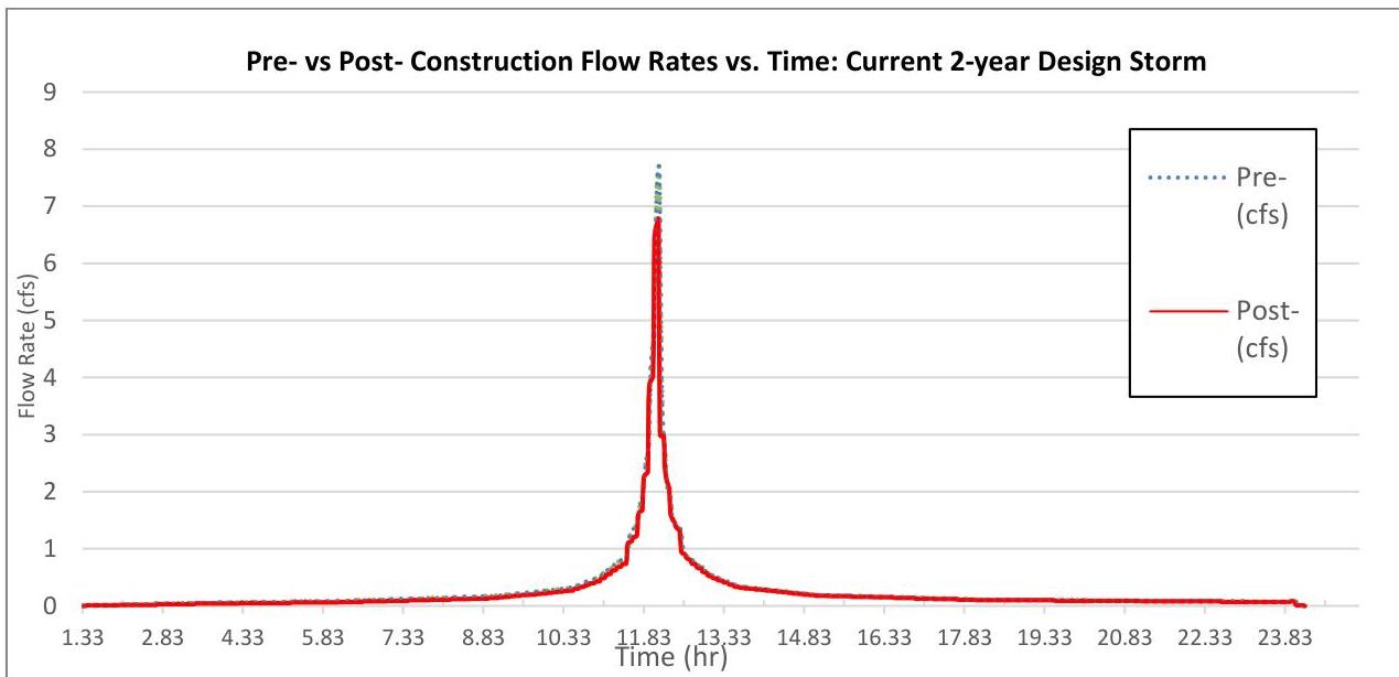
Pre- and post-condition hydrographs are provided in the chart below. As with those for the projected 100-year storm from Step 3, they appear to be nearly identical.

[OCR image]

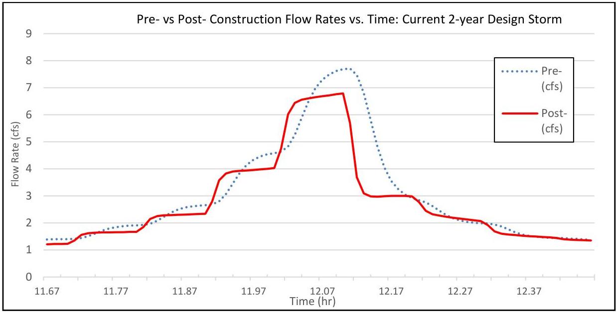
However, an analysis of the data shows several timeframes of data points where the post-construction peak flow rate exceeds the pre-construction peak flow rate. Shown below is a close up of a portion of the hydrograph with some of those time periods of exceedances.

[OCR image]

This example dispels the common misconception that the reduction of impervious surface will automatically me

PDF page 46, image 2

Mistral ID: img-27.jpeg. Extraction bundle(s): 2023_BMP_5_SWM_Standards_and_Computations. Original page | Image file

Surrounding OCR excerpt:

data points where the post-construction peak flow rate exceeds the pre-construction peak flow rate. Shown below is a close up of a portion of the hydrograph with some of those time periods of exceedances.

[OCR image]

This example dispels the common misconception that the reduction of impervious surface will automatically meet the quantity control requirements. Municipal review engineers must require that the design report include hydrologic modelling and hydrographs even when the design engineer claims there is reduction of impervious surface by the proposed development. To reiterate, the rules do not allow a “de

PDF page 61, image 1

Mistral ID: img-28.jpeg. Extraction bundle(s): 2023_BMP_5_SWM_Standards_and_Computations. Original page | Image file

Surrounding OCR excerpt:

[OCR image]

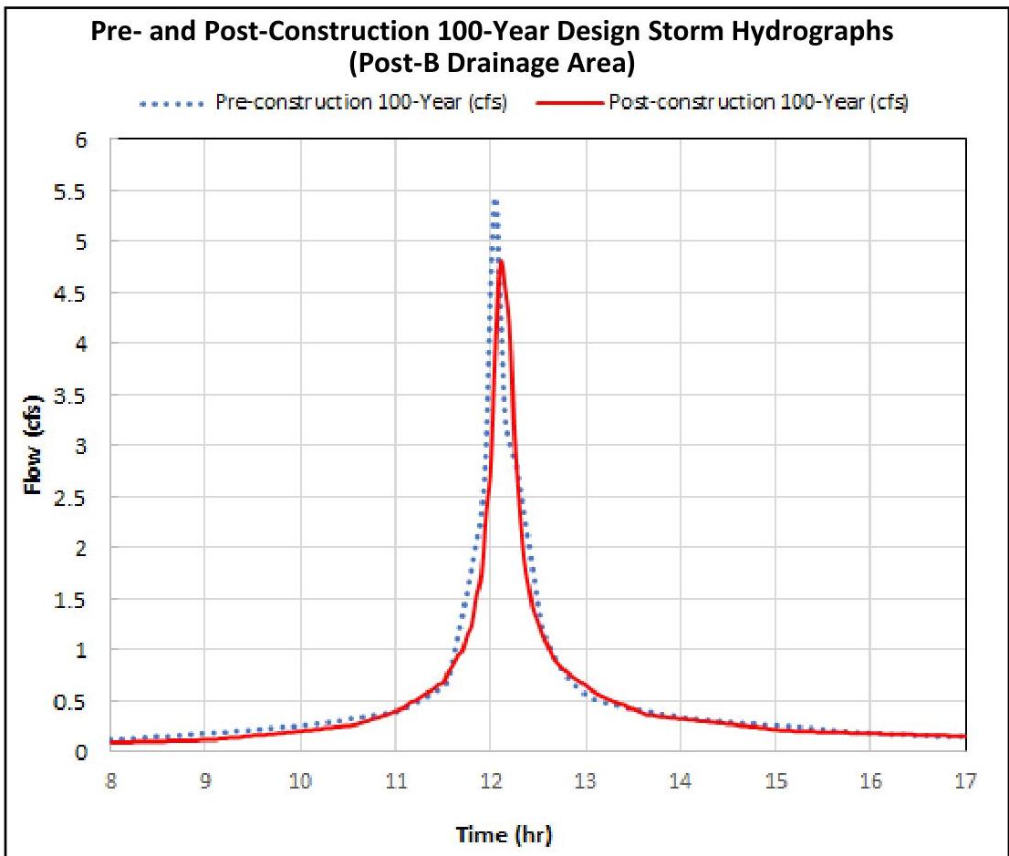
A detailed look at the flow rates generated between 12 and 13 hours is provided in a table found on the next page. Note that the flow rates in the table are from a combined hydrograph of drainage area B that is obtained by superposing runoff hydrographs of subdrainage areas B1 and B2 at the same time scale. Therefore, the peak flow rate may be different from the arithmetic sum of the peak flow rates o

PDF page 63, image 1

Mistral ID: img-29.jpeg. Extraction bundle(s): 2023_BMP_5_SWM_Standards_and_Computations. Original page | Image file

Surrounding OCR excerpt:

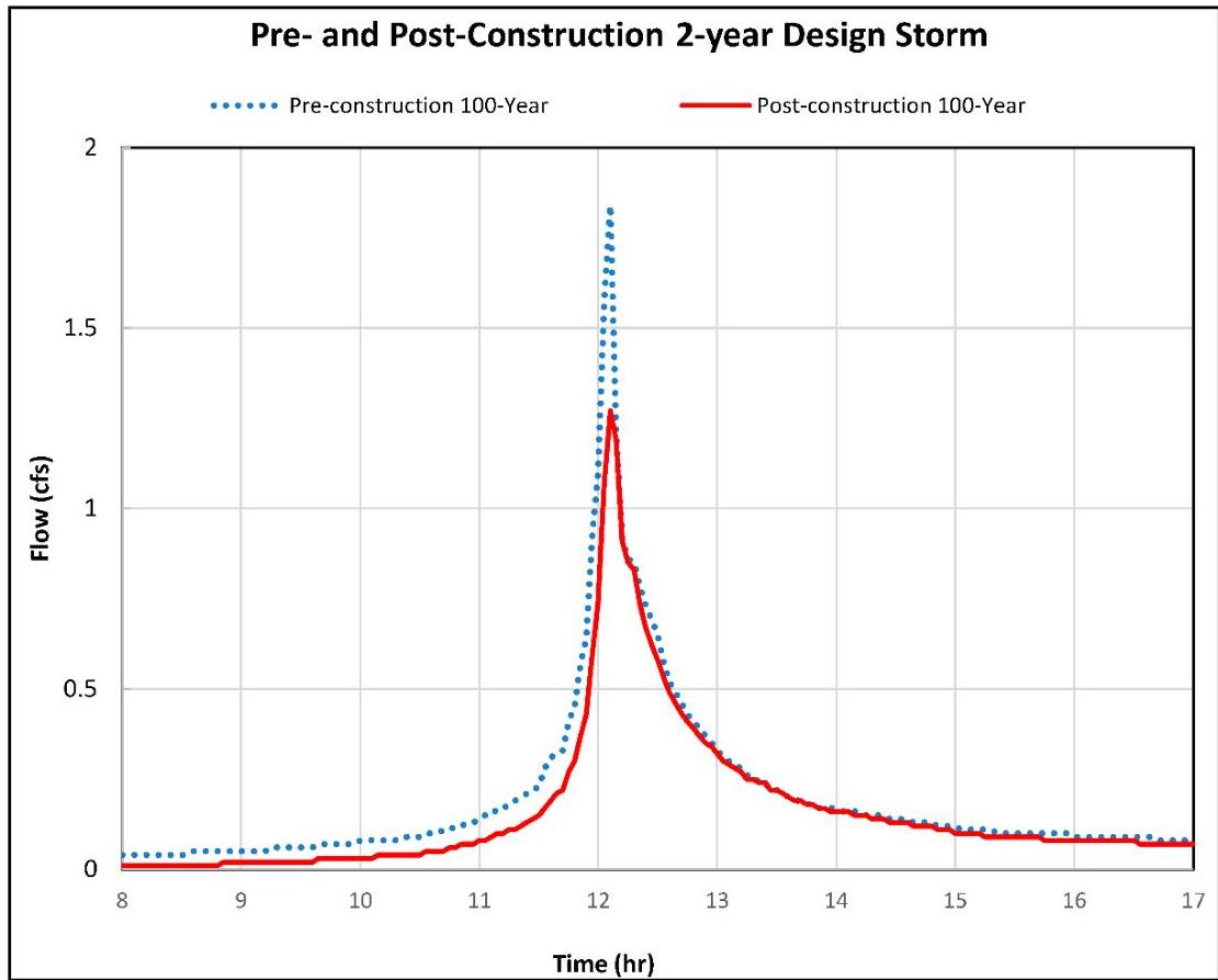
since the post-construction hydrograph for the entire site appears to not exceed the pre-construction hydrograph.

[OCR image]

Furthermore, it would be incorrect to state that areas Post-A and Post-B – combined – meet the Stormwater Runoff Quantity Control Standards of N.J.A.C. 7:8-5.6(b)1 for the 2-year design storm and those of N.J.A.C. 7:8-5.6(b)3 for the 10- and 100-year design storms. N.J.A.C. 7:8-5.2(l) requires

If there is more than one drainage area, the groundwater recharge, stormwater runoff quality, and stormwater

PDF page 67, image 1

Mistral ID: img-30.jpeg. Extraction bundle(s): 2023_BMP_5_SWM_Standards_and_Computations. Original page | Image file

Surrounding OCR excerpt:

[OCR image]

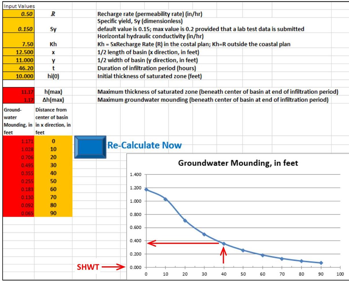
The groundwater mounding curve shows that within 40 ft from the center of the proposed small-scale bioretention (27.5 ft from the edge of the basin), the groundwater level will be elevated by approximately 0.36 ft, or roughly 7.64 ft below the existing ground elevation when the mounding under the center of the basin reaches maximum height. Note that the curve shows the mounding height at the time when

PDF page 71, image 1

Mistral ID: img-31.jpeg. Extraction bundle(s): 2023_BMP_5_SWM_Standards_and_Computations. Original page | Image file

Surrounding OCR excerpt:

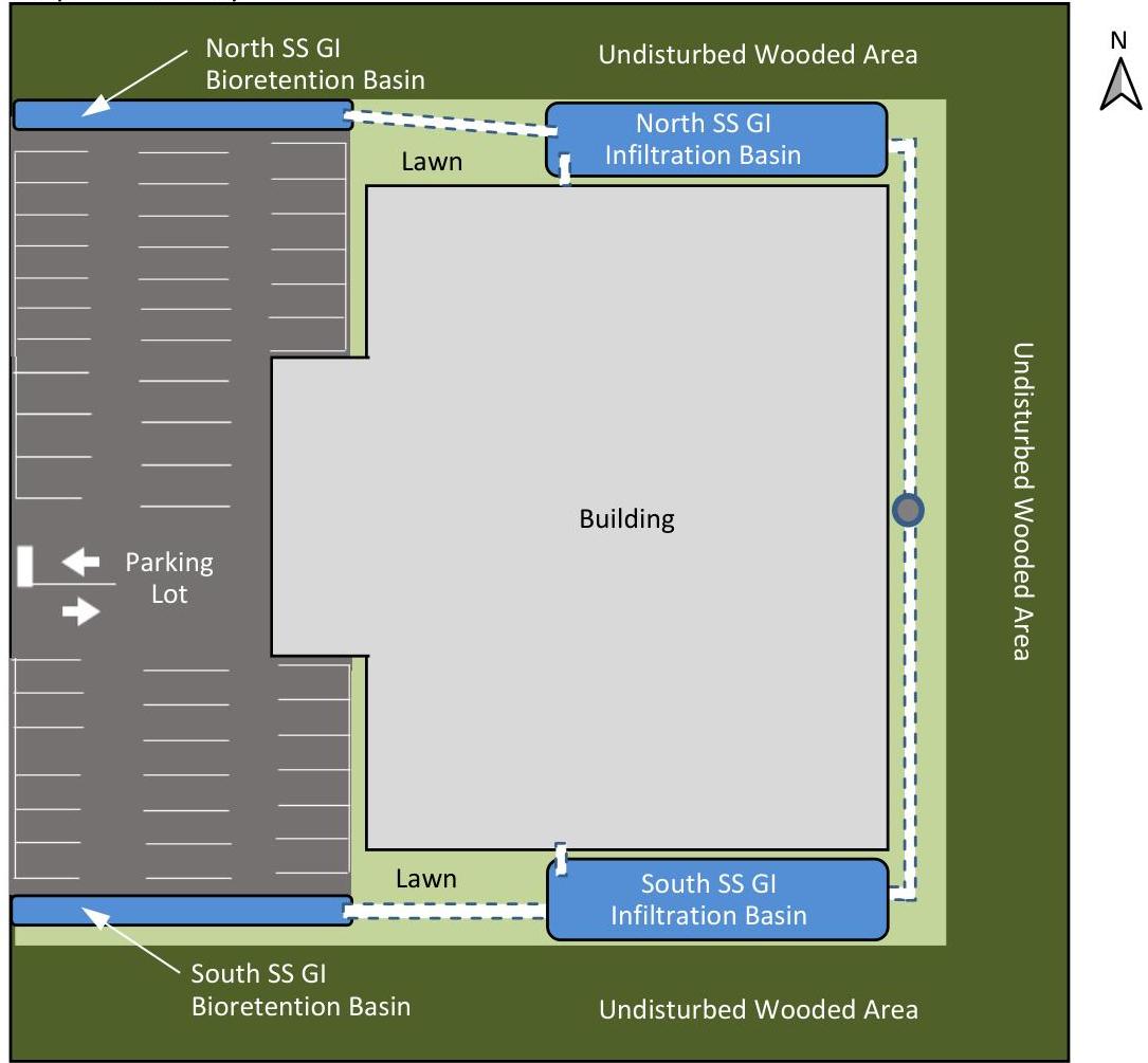
rovide water quantity control and groundwater recharge for the entire site. A proposed site layout and stormwater routing diagram are shown below; however, the drawing is not to scale.

Proposed Site Layout
[OCR image]
Note: Not to Scale

PDF page 72, image 1

Mistral ID: img-32.jpeg. Extraction bundle(s): 2023_BMP_5_SWM_Standards_and_Computations. Original page | Image file

Surrounding OCR excerpt:

ibution is used.
c. The SCS Standard DUH shall be used because the site lies outside of the coastal plain.
d. Exfiltration is not used in this design example.

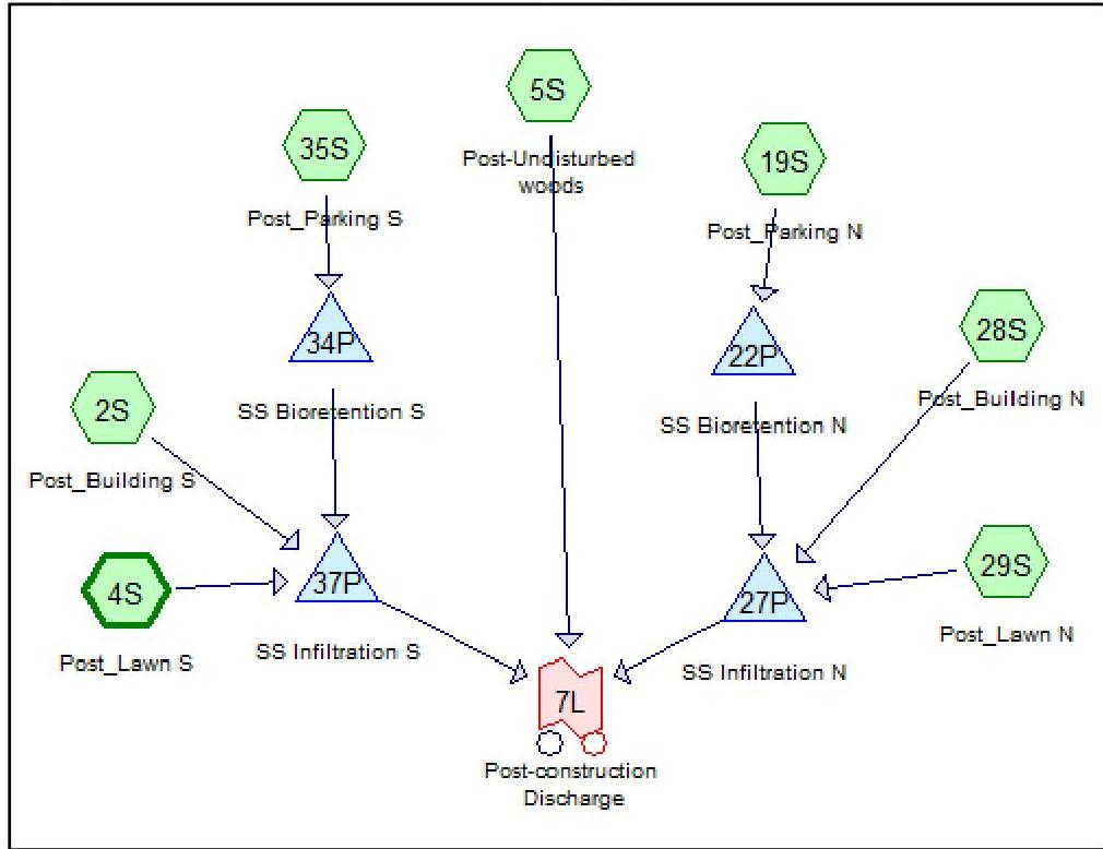
Proposed Condition Stormwater Routing Diagram

[OCR image]

Source: HydroCAD® Diagram; HydroCAD is a registered trademark of HydroCAD Software Solutions LLC. Used with permission.

Take note that the selections and configurations of the BMPs used to meet the green infrastructure, water quality, water quantity and groundwater recharge standards are for example purposes only and are not to be interpreted as the only way to design stormwater management measures.

PDF page 79, image 1

Mistral ID: img-33.jpeg. Extraction bundle(s): 2023_BMP_5_SWM_Standards_and_Computations. Original page | Image file

Tables on the same PDF page: Table 50

Surrounding OCR excerpt:

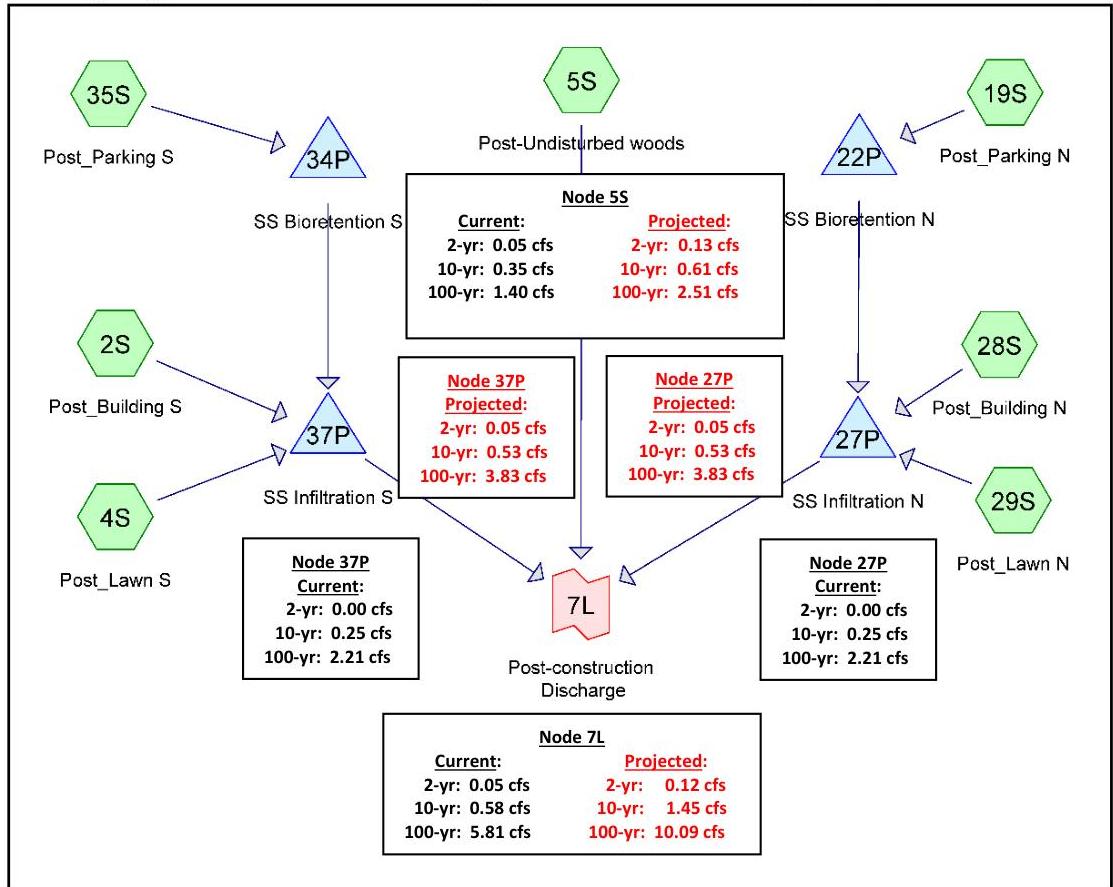
Routing Diagram with Current and Projected Peak Flow Rates Superimposed
[OCR image]
Source: HydroCAD® Diagram; HydroCAD is a registered trademark of HydroCAD Software Solutions LLC. Used with permission. Each numbered element is called a "node."

|  Post-Construction Condition Off-Site Discharges  |   |   |   |   |
| --- | --- | --- | --- | --- |
|  Design Storm | Current Precipitation Peak Flow Rate (cfs) |   | Projected Precipitation Peak Flow Rate (cfs)  |   |
|   |  Total Allowabl